[GSP077] TensorFlow for Poets

https://www.qwiklabs.com/focuses/1095?parent=catalog

Overview

TensorFlow is an open source library for numerical computation, specializing in machine learning applications. In this lab you will learn how to install and run TensorFlow on a single machine, then train a simple classifier to classify images of flowers.

Introduction

This lab uses transfer learning to train your machine. In transfer learning, when you build a new model to classify your original dataset, you reuse the feature extraction part and re-train the classification part with your dataset. This method uses less computational resources and training time. Deep learning from scratch can take days, but transfer learning can be done in short order.

The model for this lab is trained on the ImageNet Large Visual Recognition Challenge dataset. These models can differentiate between 1,000 different classes, like “Zebra”, “Dalmatian”, and “Dishwasher”. In a production environment, you’ll have a choice of model architectures, so you can determine the right tradeoff between speed, size, and accuracy for your problem.

At the end of the lab you’ll have the opportunity to retrain the same model to tell apart a small number of classes based on your own examples.

What you will learn:

• How to use Python and TensorFlow to train an image classifier
• How to classify images with your trained classifier

What you need:

• A basic understanding of Linux commands
• Your own images of flowers to upload into the lab

Create a development machine in Compute Engine

Compute Engine > VM Instances > Create

Name: devhost
Region: us-central1
Zone: us-central1-a
Machine Type: 4 vCPUs (n1-highcpu-4) instance
Boot disk: Click Change, then select Ubuntu 16.04 LTS, then click Select
Identity and API Access: "Allow full access to all Cloud APIs"

devhost > SSH

Install TensorFlow

$ sudo apt-get update
$ sudo apt-get install -y python-pip python-dev

$ sudo pip  install --upgrade https://storage.googleapis.com/tensorflow/linux/cpu/tensorflow-1.4.0-cp27-none-linux_x86_64.whl

$ python

>>> import tensorflow as tf
>>> hello = tf.constant('Hello, TensorFlow!')
>>> sess = tf.Session()
>>> print(sess.run(hello))
>>> exit

Clone the git repository

$ git clone https://github.com/googlecodelabs/tensorflow-for-poets-2
$ cd tensorflow-for-poets-2

Download the training images

Before you start any training, you’ll need a set of images to teach the model about the new classes you want to recognize. We’ve created an archive of creative-commons licensed flower photos to use initially. Download the photos (218 MB) by invoking the following commands in the SSH:

$ curl http://download.tensorflow.org/example_images/flower_photos.tgz \
| tar xz

$ mv flower_photos tf_files

(Re)training the network

Configure your MobileNet

The retrain script can retrain either Inception V3 model or a MobileNet. In this lab you will use a MobileNet. The principal difference is that Inception V3 is optimized for accuracy, while the MobileNets are optimized to be small and efficient, at the cost of some accuracy.

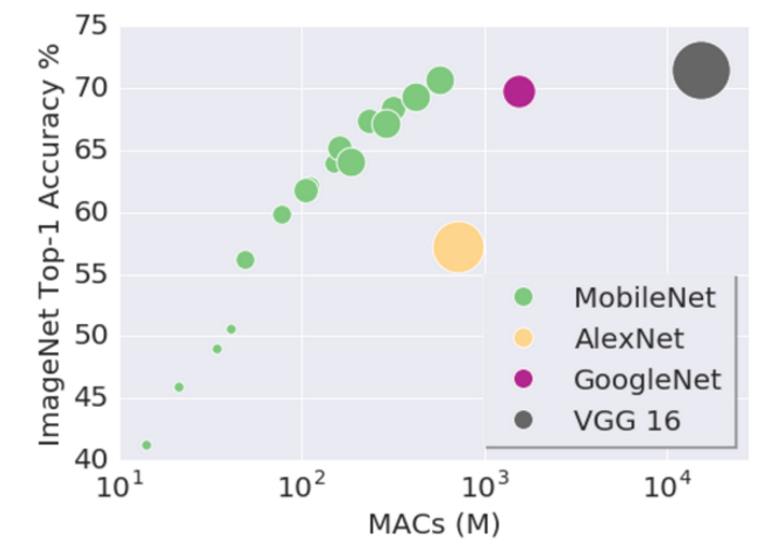
Inception V3 has a first-choice accuracy of 78% on ImageNet, but the model is 85MB, and requires many times more processing than even the largest MobileNet configuration, which achieves 70.5% accuracy, with just a 19MB download.

The following configuration options are available:

• Input image resolution: 128,160,192, or 224px. Unsurprisingly, feeding in a higher resolution image takes more processing time, but results in better classification accuracy. We recommend 224 as an initial setting.
• The relative size of the model as a fraction of the largest MobileNet: 1.0, 0.75, 0.50, or 0.25. We recommend 0.5 as an initial setting. The smaller models run significantly faster, at a cost of accuracy.

With the recommended settings, it typically takes only a couple of minutes to retrain on a laptop.

For this lab you’ll use the highest settings. In the SSH window, pass the settings inside Linux shell variables with the following commands:

$ export IMAGE_SIZE=224
$ export ARCHITECTURE="mobilenet_0.50_${IMAGE_SIZE}"

The graph below shows the first-choice-accuracies of these configurations (y-axis), vs the number of calculations required (x-axis), and the size of the model (circle area).

16 points are shown for MobileNet. For each of the 4 model sizes (circle area in the figure) there is one point for each image resolution setting. The 128px image size models are represented by the lower-left point in each set, while the 224px models are in the upper right.

Open a firewall for Tensorboard on port 6006

TensorBoard is a monitoring and inspection tool included with TensorFlow. You will use it to monitor the training progress. In order for your VM to get to TensorBoard, you’ll create a firewall rule.

In the Console, click on devhost.

Scroll down and under Network Interfaces, click on default under the Network heading.

Firewall Rules > “Create Firewall Rule”

Name: tensorboard
Targets: All instances in the network
Source IP ranges: 0.0.0.0/0
Protocol and ports: check tcp, and then type "6006"

Start TensorBoard

$ tensorboard --logdir tf_files/training_summaries &

Navigation menu > Compute Engine > VM instances.

Посмотреть

Run the training

As noted in the introduction, Imagenet models are networks with millions of parameters that can differentiate a large number of classes. We’re only training the final layer of that network, so training will end in a reasonable amount of time.

In the SSH, start your retraining with one big command (note the –summaries_dir option, sending training progress reports to the directory that tensorboard is monitoring):

$ python -m scripts.retrain \
  --bottleneck_dir=tf_files/bottlenecks \
  --how_many_training_steps=500 \
  --model_dir=tf_files/models/ \
  --summaries_dir=tf_files/training_summaries/"${ARCHITECTURE}" \
  --output_graph=tf_files/retrained_graph.pb \
  --output_labels=tf_files/retrained_labels.txt \
  --architecture="${ARCHITECTURE}" \
  --image_dir=tf_files/flower_photos

This script downloads the pre-trained model, adds a new final layer, and trains that layer on the flower photos you’ve downloaded to the lab.

ImageNet does not include any of these flower species you’re training on. The kinds of information that make it possible for ImageNet to differentiate among 1,000 classes are useful for distinguishing other objects. By using this pre-trained network, you’re using that information as input to the final classification layer that distinguishes your flower classes.

This will take several minutes to complete. Read through the next couple of sections while the training is running.

More about Bottlenecks

This section and the next provide background on how this retraining process works.

The first phase analyzes all the images on disk and calculates the bottleneck values for each of them. What’s a bottleneck?

These ImageNet models are made up of many layers stacked on top of each other, a simplified picture of Inception V3 from TensorBoard, is shown above (all the details are available in this paper, with a complete picture on page 6). These layers are pre-trained and are already very valuable at finding and summarizing information that will help classify most images. For this lab, you are training only the last layer (final_training_ops in the figure below). While all the previous layers retain their already-trained state.

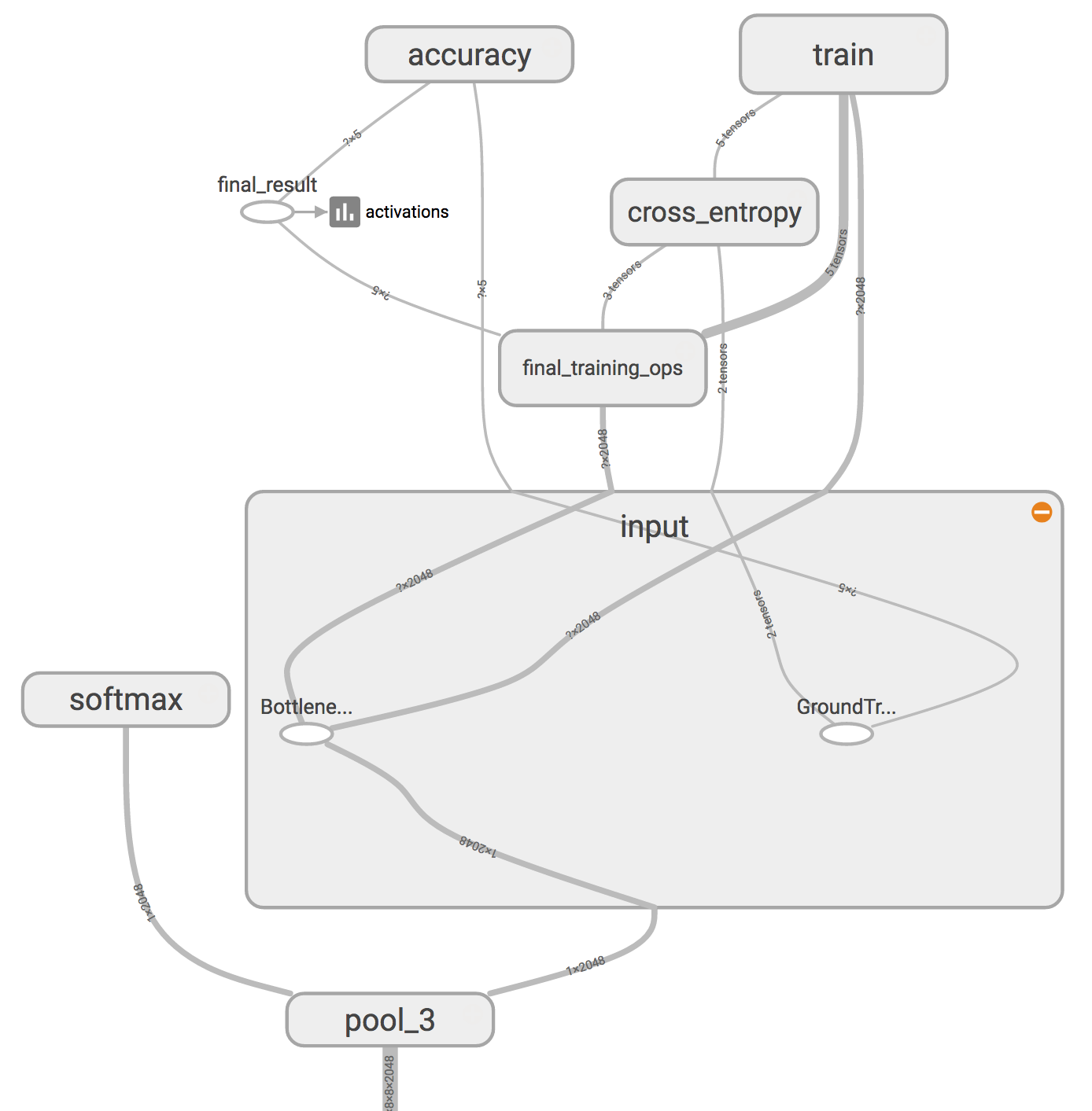
In the above figure, the node labeled “softmax”, on the left side, is the output layer of the original model. All the nodes to the right of the “softmax” were added by the retraining script.

A bottleneck is an informal term often used for the layer just before the final output layer that actually does the classification. “Bottelneck” is not used to imply that the layer is slowing down the network, but because near the output, the representation is much more compact than in the main body of the network.

Every image is reused multiple times during training. Calculating the layers behind the bottleneck for each image takes a significant amount of time. Since these lower layers of the network are not being modified their outputs can be cached and reused.

So the script is running the constant part of the network, everything below the node labeled Bottlene… above, and caching the results.

The command you ran saves these files to the bottlenecks/ directory. If you rerun the script, they’ll be reused, so you don’t have to wait for this part again.

More about Training

Once the script finishes generating all the bottleneck files, the actual training of the final layer of the network begins.

The training operates efficiently by feeding the cached value for each image into the Bottleneck layer. The true label for each image is also fed into the node labeled GroundTruth. Just these two inputs are enough to calculate the classification probabilities, training updates, and the various performance metrics.

As it trains you’ll see a series of step outputs, each one showing training accuracy, validation accuracy, and the cross entropy:

• The training accuracy shows the percentage of the images used in the current training batch that were labeled with the correct class.
• Validation accuracy is the precision (percentage of correctly-labelled images) on a randomly-selected group of images from a different set.
• Cross entropy is a loss function that gives a glimpse into how well the learning process is progressing (lower numbers are better here).

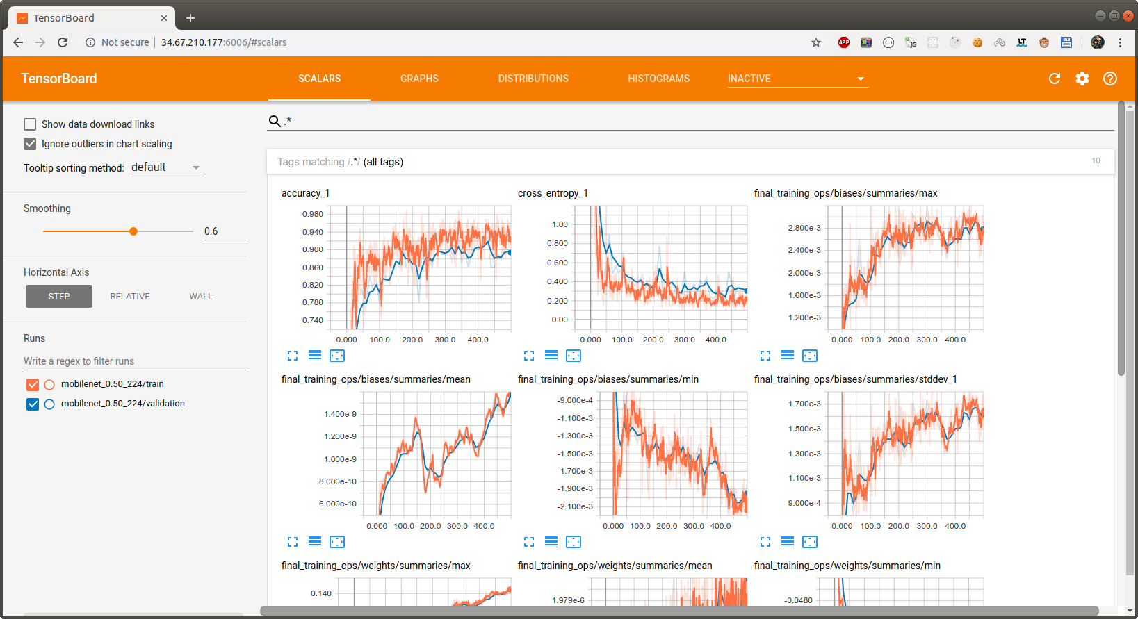
The figures below show an example of the progress of the model’s accuracy and cross entropy as it trains. When your model has finished generating the bottleneck files you can check your model’s progress by opening TensorBoard, and clicking on the figure’s name to show them. TensorBoard may print out warnings to your command line. These can safely be ignored.

A true measure of the performance of the network is to measure its performance on a data set that is not in the training data. This performance is measured using the validation accuracy. If the training accuracy is high but the validation accuracy remains low, that means the network is overfitting, and the network is memorizing particular features in the training images that don’t help it classify images more generally.

The training’s objective is to make the cross entropy as small as possible, so you can tell if the learning is working by keeping an eye on whether the loss keeps trending downwards, ignoring the short-term noise.

By default, this script runs 4,000 training steps. Each step chooses 10 images at random from the training set, finds their bottlenecks from the cache, and feeds them into the final layer to get predictions. Those predictions are then compared against the actual labels to update the final layer’s weights through a backpropagation process.

As the process continues, you should see the reported accuracy improve. After all the training steps are complete, the script runs a final test accuracy evaluation on a set of images that are kept separate from the training and validation pictures. This test evaluation provides the best estimate of how the trained model will perform on the classification task.

You should see an accuracy value of between 85% and 99%, though the exact value will vary from run to run since there’s randomness in the training process. (If you are only training on two classes, you should expect higher accuracy.) This number value indicates the percentage of the images in the test set that are given the correct label after the model is fully trained.

Go back to TensorBoard tab

When the command line returns that means that the training is complete. Go look at the TensorBoard tab again to see what your results look like.

Using the Retrained Model

The retraining script writes data to the following two files:

• tf_files/retrained_graph.pb, which contains a version of the selected network with a final layer retrained on your categories.
• tf_files/retrained_labels.txt, which is a text file containing labels.

Classifying an image

Next you will run the script on this image of a daisy:

flower_photos/daisy/21652746_cc379e0eea_m.jpg Image CC-BY by Retinafunk

$ python -m scripts.label_image \
    --graph=tf_files/retrained_graph.pb  \
    --image=tf_files/flower_photos/daisy/21652746_cc379e0eea_m.jpg

Each execution will print a list of flower labels, in most cases with the correct flower on top (though each retrained model may be slightly different).

You should get results like this for the daisy photo:

daisy (score=0.99234)
dandelion (score=0.00693)
sunflowers (score=0.00070)
roses (score=0.00003)
tulips (score=0.00000)

This indicates a high confidence (~99%) that the image is a daisy, and low confidence for any other label.

Try it again with a new image:

flower_photos/roses/2414954629_3708a1a04d.jpg Image CC-BY by Lori Branham

$ python -m scripts.label_image \
    --graph=tf_files/retrained_graph.pb  \
    --image=tf_files/flower_photos/roses/2414954629_3708a1a04d.jpg

roses (score=0.93928)
tulips (score=0.06065)
dandelion (score=0.00005)
daisy (score=0.00001)
sunflowers (score=0.00001)