[GSP140] Using Distributed TensorFlow with Cloud ML Engine and Cloud Datalab

https://www.qwiklabs.com/focuses/1254?parent=catalog

Overview

This lab shows you how to use a distributed configuration of TensorFlow code in Python on Google Cloud Machine Learning Engine to train a convolutional neural network model by using MNIST—a dataset that is widely used in machine learning training to recognize handwritten digits. You will be using TensorBoard to visualize the training process and Google Cloud Datalab to test predictions.

TensorFlow is Google’s open source library for machine learning, developed by researchers and engineers in Google’s Machine Intelligence organization, which is part of Research at Google. TensorFlow is designed to run on multiple computers to distribute the training workloads, and Cloud Machine Learning Engine provides a managed service where you can run TensorFlow code in a distributed manner by using service APIs.

Understanding Neural Networks

In computer programming, humans instruct a computer to solve a problem by specifying each step using many lines of code. Machine learning and neural networks on the other hand teach a computer to solve problems by feeding it examples. Many examples.

In computing terms, a neural network is a mathematical function that can learn the expected output for a given input by training datasets. The following figure illustrates a neural network that has been trained to output “cat” from a cat image.

You can see that a neural network model consists of multiple layers of calculation units, in which each layer has configurable parameters. The goal of training the model is to optimize the parameters to get results with the highest accuracy. The training algorithm makes adjustments as it processes batches of training datasets through the model. If you distribute the training process to multiple computational nodes, you need a way to keep track of the changing parameters to be shared by all nodes.

Architecture of the distributed training

There are three basic strategies to train a model with multiple nodes (or application containers that run parallel computations):

• Data-parallel training with synchronous updates.
• Data-parallel training with asynchronous updates.
• Model-parallel training.

The example code in this Qwiklab uses data-parallel training with asynchronous updates on Cloud ML Engine. In this case, a training job is executed using the following types of nodes:

• Parameter server node: updates parameters with gradient vectors from worker and chief work nodes.
• Worker node: calculates a gradient vector from the training dataset.
• Chief worker node: coordinate the operations of multiple workers, in addition to working as one of the worker nodes.

Because you can use the data-parallel strategy regardless of the model structure, it is a good starting point for applying the distributed training method to your custom model. In data-parallel training, the whole model is shared with all worker nodes. Each node calculates gradient vectors independently from some part of the training dataset in the same manner as the mini-batch processing. The calculated gradient vectors are collected into the parameter server node, and model parameters are updated with the total summation of the gradient vectors. If you distribute 10,000 batches among 10 worker nodes, each node works on roughly 1,000 batches.

Data-parallel training can be done with either synchronous or asynchronous updates. When using asynchronous updates, the parameter server applies each gradient vector independently, right after receiving it from one of the worker nodes, as shown in the following diagram:

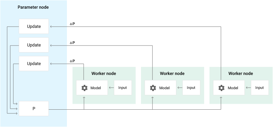
In a typical deployment, there are a few parameter server nodes, a single chief worker node, and several worker nodes. When you submit a training job through the service API, these nodes are automatically deployed in your project.

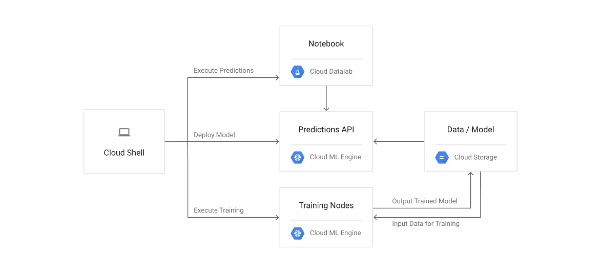
The following diagram describes the architecture for running a distributed training job on Cloud ML Engine and using Cloud Datalab to execute predictions with your trained model.

Objectives

Now that we have a better understanding of the theory behind neural networks and distributed training, let’s go over what you’ll do in this lab:

• Run the distributed TensorFlow sample code on Cloud ML Engine.
• Deploy the trained model to Cloud ML Engine to create a custom API for predictions.
• Visualize the training process with TensorBoard.
• Use Cloud Datalab to test the predictions.

Preparing the Environment

This Qwiklab uses Cloud Shell, a fully functioning Linux shell in the Google Cloud Platform Console to run commands.

Open a Cloud Shell instance and run the following command to list Cloud ML models (verify that the command returns 0 items):

$ gcloud ml-engine models list

Now let’s clone the MNIST GitHub repository:

$ git clone https://github.com/GoogleCloudPlatform/cloudml-dist-mnist-example

$ cd cloudml-dist-mnist-example

Great! We have all the MNIST files we need to train our models.

Creating a Cloud Storage Bucket for MNIST Files

Now that we’ve downloaded the proper files, let’s create a Cloud Storage bucket to hold the MNIST data used to train the model.

Run the following command:

$ PROJECT_ID=$(gcloud config list project --format "value(core.project)")

$ MNIST_BUCKET="${PROJECT_ID}-ml"

$ gsutil mb -c regional -l us-east1 gs://${MNIST_BUCKET}

Use the following script to download the MNIST data files and copy them to the bucket:

$ sudo ./scripts/create_records.py

$ gsutil cp /tmp/data/train.tfrecords gs://${MNIST_BUCKET}/data/

$ gsutil cp /tmp/data/test.tfrecords gs://${MNIST_BUCKET}/data/

Training the model on Cloud Machine Learning Engine

Run the following command to submit a training job to Cloud ML Engine:

$ JOB_NAME="job_$(date +%Y%m%d_%H%M%S)"

$ gcloud ml-engine jobs submit training ${JOB_NAME} \
    --package-path trainer \
    --module-name trainer.task \
    --staging-bucket gs://${MNIST_BUCKET} \
    --job-dir gs://${MNIST_BUCKET}/${JOB_NAME} \
    --runtime-version 1.2 \
    --region us-central1 \
    --config config/config.yaml \
    -- \
    --data_dir gs://${MNIST_BUCKET}/data \
    --output_dir gs://${MNIST_BUCKET}/${JOB_NAME} \
    --train_steps 5000

The –train_steps option specifies the total number of training batches.

You can control the amount of resources allocated for the training job by specifying a scale tier with the configuration file config/config.yaml. When the job starts running on multiple nodes, the same Python code in the trainer directory that is specified with –package-path parameter are deployed on all nodes. The files in the trainer directory and their functions are listed in the table below:

setup.py - Setup script to install additional modules on nodes.

model.py - TensorFlow code to define the convolutional neural network model.

task.py - TensorFlow code to run the training task. In this example, Experiment API is used to run the training loop in a distributed manner.

AI Platform > Jobs.

While the job is running, click on the “View Logs” link.

The example code shows progress in logs during the training. You will see some warnings and errors for around 5 minutes as the nodes are initialized but the scripts will report progress periodically as the training data set is processed. For example, each worker node shows a training loss value, which represents the total loss value for the dataset in a single training batch, at some intervals. In addition, the chief worker node shows a loss and accuracy for the test set. At the end of the training, the final evaluation against the test set is shown. In this example, the training achieved 98.7% accuracy for the test set.

The training task will take approximately 15 minutes to complete. In the logs, you’ll see this a log like this:

Saving dict for global step 5008: accuracy = 0.987, global_step = 5008, loss = 0.0466603

You can even search for “saving dict for global” if the log isn’t readily visible. After the training, the trained model is exported in the storage bucket. You can find the storage path for the directory that contains the model binary by using the following command:

$ gsutil ls gs://${MNIST_BUCKET}/${JOB_NAME}/export/Servo | tail -1

The output should look like this:

// $ gs://${MNIST_BUCKET}/job_[TIMESTAMP]/export/Servo/[JOB_ID]/:
gs://qwiklabs-gcp-7fbe07df92cae882-ml/job_20190617_204501/export/Servo/1560794260/

Visualizing the training process with TensorBoard

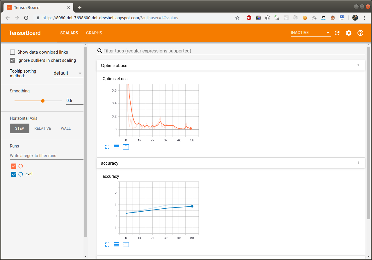
After the training, the summary data is stored in gs://${MNIST_BUCKET}/${JOB_NAME}. You will know visualize the data with TensorBoard.

Run the following command in Cloud Shell to start TensorBoard:

$ tensorboard --port 8080 --logdir gs://${MNIST_BUCKET}/${JOB_NAME}

To open a new browser window, select Preview on port 8080 from the Web preview menu in the top-right corner of the Cloud Shell toolbar.

In the new window, you can use TensorBoard to see the training summary and the visualized network graph.

Deploying the trained model for predictions

You deploy the trained model for predictions using the model binary.

Deploy the model and set the default version.

$ MODEL_NAME=MNIST

$ gcloud ml-engine models create --regions us-central1 ${MODEL_NAME}
VERSION_NAME=v1

$ ORIGIN=$(gsutil ls gs://${MNIST_BUCKET}/${JOB_NAME}/export/Servo | tail -1)

$ gcloud ml-engine versions create \
    --origin ${ORIGIN} \
    --runtime-version=1.2 \
    --model ${MODEL_NAME} \
    ${VERSION_NAME}

$ gcloud ml-engine versions set-default --model ${MODEL_NAME} ${VERSION_NAME}

These commands will take about five minutes to complete.

MODEL_NAME and VERSION_NAME can be arbitrary, but you can’t reuse the same name. The last command is not necessary in this case, as the first version automatically becomes the default, but it’s a good practice to set the default explicitly.

It might take a few minutes for the deployed model to become ready. Until it becomes ready, it returns an HTTP 503 error against requests.

Test the prediction API by using a sample request file.

$ ./scripts/make_request.py

This script creates a JSON file, named request.json, containing 10 test images for predictions.

Submit an online prediction request.

$ gcloud ml-engine predict --model ${MODEL_NAME} --json-instances request.json

You should get a response that looks something like this:

CLASSES  PROBABILITIES
7        [7.127025003690092e-15, ... 3.894632616407989e-09]
2        [2.1343875018092762e-13, ... 3.4817655638637703e-15]
1        [4.6818767612810674e-11, ... 8.201765377968684e-10]
0        [1.0, 9.028149372704427e-16, ... 2.4338968340753553e-12]
4        [3.43453356033141e-11, ... 1.7647047343416489e-06]
1        [9.1312964134449e-12, ... 9.780157239624998e-11]
4        [5.647431578371248e-14, ... 3.3598115578570287e-07]
9        [5.707836005057476e-13, ... 0.9999985694885254]
5        [2.0792810528913463e-10, ... 8.556835240369765e-08]
9        [7.901934895430702e-16, ... 1.0]

CLASSES is the most probable digit of the given image, and PROBABILITIES shows the probabilities of each digit.

Executing predictions with Cloud Datalab

To test your predictions, create a Cloud Datalab instance that uses interactive Jupyter Notebooks to execute code.

In Cloud Shell, enter the following command to create a Cloud Datalab instance:

$ datalab create mnist-datalab --zone us-central1-a

This will take a few minutes to complete.

You will see a warning stating that “This tool needs to create the directory…” before it can generate the SSH keys.

For the passphrase prompt you can just press Enter twice to use a blank passphrase for this lab.

When you see the Click on the “Web Preview” message appear in Cloud Shell, launch the Cloud Datalab notebook listing page by clicking Cloud Shell Web preview using the square icon in the top right of the Cloud Shell tab.

Select Change port, type in 8081 then Change and Preview to launch a new tab in your browser.

In the Cloud Datalab application, create a new notebook by clicking on the +Notebook icon in the upper left make sure you are in /datalab directory.

Paste the following text into the first cell of the new notebook:

%%bash
wget https://raw.githubusercontent.com/GoogleCloudPlatform/cloudml-dist-mnist-example/master/notebooks/Online%20prediction%20example.ipynb
cat Online\ prediction\ example.ipynb > Untitled\ Notebook.ipynb

Click Run at the top of the page to download the Online prediction example.ipynb notebook. The script copies the remote notebook’s contents into the current notebook.

Refresh the browser page to load the new notebook content.

Scroll down to the first cell that contains JavaScript clod and click on it. Then click Run to execute it.

Scroll down the page until you see the number drawing panel, and draw a number with your cursor:

У меня цифры не отразились. Далее copy+paste без проверок.

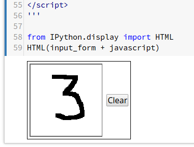
Click in the next cell below the the number drawing panel to activate it. Click on the down arrow next to the Run button at the top and select Run from this Cell.

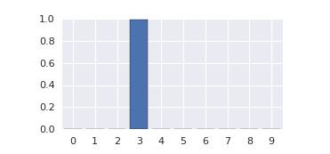
The output of the prediction is a length-10 array in which each index, 0-9, contains a number corresponding to that digit. The closer the number is to 1, the more likely that index matches the digit you entered. You can see that the fourth slot, which corresponds to the number 3, highlighted in the list below is very close to 1, and therefore has a high probability of matching the digit.

PROBABILITIES
[4.181503356903704e-07, 7.12400151314796e-07, 0.00017898145597428083, 0.9955494403839111, 5.323939553103507e-11, 0.004269002005457878, 7.927398321116996e-11, 1.2688398953741853e-07, 1.0825967819982907e-06, 2.2037748692582682e-07]

The last cell in the notebook displays a bar chart that clearly shows that it recognized your number, which was 3 in this case.