[GSP271] Machine Learning with Spark on Google Cloud Dataproc
https://www.qwiklabs.com/focuses/3390?parent=catalog
This lab uses a set of code samples and scripts developed for Chapter 7, Machine Learning: Logistic Regression on Spark, from the Data Science on Google Cloud Platform book from O’Reilly Media, Inc.
Note: The automated lab setup process for this lab pre-creates a Google Cloud Storage bucket for you that is named using the project ID. This storage bucket includes a number of data files that are used here and will be used again later in the lab.
Overview
In this lab you will learn how to implement logistic regression using a machine learning library for Apache Spark running on a Google Cloud Dataproc cluster to develop a model for data from a multivariable dataset.
Google Cloud Dataproc is a fast, easy-to-use, fully-managed cloud service for running Apache Spark and Apache Hadoop clusters in a simple, cost-efficient way. Cloud Dataproc easily integrates with other Google Cloud Platform (GCP) services, giving you a powerful and complete platform for data processing, analytics and machine learning
Apache Spark is an analytics engine for large scale data processing. Logistic regression is available as a module in Apache Spark’s machine learning library, MLlib. Spark MLlib, also called Spark ML, includes implementations for most standard machine learning algorithms such as k-means clustering, random forests, alternating least squares, k-means clustering, decision trees, support vector machines, etc. Spark can run on a Hadoop cluster, like Google Cloud Dataproc, in order to process very large datasets in parallel.
The base data set that is used provides historical information about internal flights in the United States retrieved from the US Bureau of Transport Statistics website. This data set can be used to demonstrate a wide range of data science concepts and techniques and is used in all of the other labs in the Data Science on the Google Cloud Platform and Data Science on Google Cloud Platform: Machine Learning quests. In this lab the data is provided for you as a set of CSV formatted text files.
Objectives
- Prepare the Spark interactive shell on a Google Cloud Dataproc cluster.
- Create a training dataset for machine learning using Spark.
- Develop a logistic regression machine learning model using Spark.
- Evaluate the predictive behavior of a machine learning model using Spark on Google Cloud Datalab.
Prepare the Spark Interactive Shell
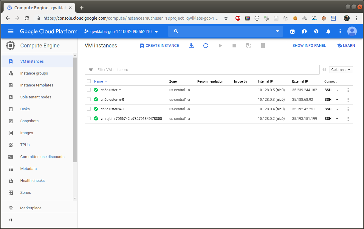
Compute Engine > VM Instances > ch6cluster-m > SSH

$ export PROJECT_ID=$(gcloud info --format='value(config.project)')
$ export BUCKET=${PROJECT_ID}
$ export ZONE=us-central1-a

$ pyspark
The SparkContext variable sc and the SparkSession variable spark are pre-configured in both the interactive Spark shell and Cloud Datalab.
Create a Spark Dataframe for Training
To get started on this lab you need to import the Logistic Regression classes.
>>> from pyspark.mllib.classification import LogisticRegressionWithLBFGS
>>> from pyspark.mllib.regression import LabeledPoint
Next, fetch the Cloud Storage bucket name from the environment variable you set earlier. Using that bucket you create the traindays DataFrame by reading in a prepared CSV that was copied into the bucket for you when the lab was launched. The CSV identifies a subset of days as valid for training. This allows you to create views of the entire flights dataset which is divided into a dataset used for training your model and a dataset used to test or validate that model. The details on how to create that CSV file are covered in earlier labs in this series.
>>> BUCKET=os.environ['BUCKET']
>>> traindays = spark.read \
      .option("header", "true") \
      .csv('gs://{}/flights/trainday.csv'.format(BUCKET))
// Make this a Spark SQL view as well to make it easier to reuse later:
>>> traindays.createOrReplaceTempView('traindays')

// Query the first few records from the training dataset view:
>>> spark.sql("SELECT * from traindays ORDER BY FL_DATE LIMIT 5").show()
This displays the first five records in the training table:
+----------+------------+
|   FL_DATE|is_train_day|
+----------+------------+
|2015-01-01|        True|
|2015-01-02|       False|
|2015-01-03|       False|
|2015-01-04|        True|
|2015-01-05|        True|
+----------+------------+
Now you create a schema for the actual flights dataset. As you have seen in previous labs, almost all of the fields in this dataset are strings apart from the four numeric fields for departure delay, taxi out time, flight distance, and arrival delay:
>>> from pyspark.sql.types \
    import StringType, FloatType, StructType, StructField

>>> header = 'FL_DATE,UNIQUE_CARRIER,AIRLINE_ID,CARRIER,FL_NUM,ORIGIN_AIRPORT_ID,ORIGIN_AIRPORT_SEQ_ID,ORIGIN_CITY_MARKET_ID,ORIGIN,DEST_AIRPORT_ID,DEST_AIRPORT_SEQ_ID,DEST_CITY_MARKET_ID,DEST,CRS_DEP_TIME,DEP_TIME,DEP_DELAY,TAXI_OUT,WHEELS_OFF,WHEELS_ON,TAXI_IN,CRS_ARR_TIME,ARR_TIME,ARR_DELAY,CANCELLED,CANCELLATION_CODE,DIVERTED,DISTANCE,DEP_AIRPORT_LAT,DEP_AIRPORT_LON,DEP_AIRPORT_TZOFFSET,ARR_AIRPORT_LAT,ARR_AIRPORT_LON,ARR_AIRPORT_TZOFFSET,EVENT,NOTIFY_TIME'


>>> raw_input

>>> def get_structfield(colname):
   if colname in ['ARR_DELAY', 'DEP_DELAY', 'DISTANCE', 'TAXI_OUT']:
      return StructField(colname, FloatType(), True)
   else:
      return StructField(colname, StringType(), True)

^D

>>> schema = StructType([get_structfield(colname) for colname in header.split(',')])
The next stage in the process is to identify the source data files.
>>> inputs = 'gs://{}/flights/tzcorr/all_flights-00004-*'.format(BUCKET)
    >>> flights = spark.read\
                .schema(schema)\
                .csv(inputs)
    >>> flights.createOrReplaceTempView('flights')
Next, create a query that uses data only from days identified as part of the training dataset:
>>> trainquery = """
SELECT
  F.DEP_DELAY,F.TAXI_OUT,f.ARR_DELAY,F.DISTANCE
FROM flights f
JOIN traindays t
ON f.FL_DATE == t.FL_DATE
WHERE
  t.is_train_day == 'True'
"""

>>> traindata = spark.sql(trainquery)
>>> traindata.head(2)
[Row(DEP_DELAY=-2.0, TAXI_OUT=26.0, ARR_DELAY=0.0, DISTANCE=677.0), Row(DEP_DELAY=-2.0, TAXI_OUT=22.0, ARR_DELAY=3.0, DISTANCE=451.0)]
// Ask Spark to provide some analysis of the dataset:
»> traindata.describe().show()
+-------+------------------+-----------------+-----------------+-----------------+
|summary|         DEP_DELAY|         TAXI_OUT|        ARR_DELAY|         DISTANCE|
+-------+------------------+-----------------+-----------------+-----------------+
|  count|            151446|           151373|           150945|           152566|
|   mean|10.726252261532164|16.11821791204508|5.310126204909073|837.4265432665208|
| stddev| 36.38718688562445|8.897148233750972|38.04559816976176|623.0449480656523|
|    min|             -39.0|              1.0|            -68.0|             31.0|
|    max|            1393.0|            168.0|           1364.0|           4983.0|
+-------+------------------+-----------------+-----------------+-----------------+
The mean and standard deviation values have been rounded to two decimal places for clarity in this table, but you will see the full floating point values on screen.
The table shows that there are some issues with the data. Not all of the records have values for all of the variables, there are different count stats for DISTANCE, ARR_DELAY, DEP_DELAY and TAXI_OUT. This happens because:
- Flights are scheduled but never depart
- Some depart but are cancelled before take off
- Some flights are diverted and therefore never arrive
These records have NULL values instead of the relevant field values and Spark’s describe function does not count them.
The best way to deal with this is to remove flights that have been cancelled or diverted using the following query:
>>> trainquery = """
SELECT
  DEP_DELAY, TAXI_OUT, ARR_DELAY, DISTANCE
FROM flights f
JOIN traindays t
ON f.FL_DATE == t.FL_DATE
WHERE
  t.is_train_day == 'True' AND
  f.CANCELLED == '0.00' AND
  f.DIVERTED == '0.00'
"""

>>> traindata = spark.sql(trainquery)
>>> traindata.describe().show()
This should output something similar to the following, indicating that you have correctly dealt with the problem:
+-------+------------------+------------------+-----------------+-----------------+
|summary|         DEP_DELAY|          TAXI_OUT|        ARR_DELAY|         DISTANCE|
+-------+------------------+------------------+-----------------+-----------------+
|  count|            150945|            150945|           150945|           150945|
|   mean|10.672973599655503|16.110821822518137|5.310126204909073|838.4892046772003|
| stddev| 36.29471283461898| 8.879085146598761|38.04559816976176|623.1392192724009|
|    min|             -39.0|               1.0|            -68.0|             31.0|
|    max|            1393.0|             168.0|           1364.0|           4983.0|
+-------+------------------+------------------+-----------------+-----------------+
Develop a Logistic Regression Model
Now you can create a function that converts a set of data points in your DataFrame into a training example. A training example contains a sample of the input features and the correct answer for those inputs. In this case, the correct answer is whether the arrival delay is less than 15 minutes and the labels that you want to use as inputs are the values for departure delay, taxi out time, and flight distance.
Enter the following in the Pyspark interactive console to create the definition for the training example function:
>>> raw_input

def to_example(raw_data_point):
  return LabeledPoint(\
              float(raw_data_point['ARR_DELAY'] < 15), # on-time? \
              [ \
                  raw_data_point['DEP_DELAY'], \
                  raw_data_point['TAXI_OUT'], \
                  raw_data_point['DISTANCE'], \
              ])

^D
You can now map this training example function to the training dataset using a mapping:
>>> examples = traindata.rdd.map(to_example)
This gives you a training DataFrame for the Spark logistic regression module that will create a logistic regression model based on your training dataset:
>>> lrmodel = LogisticRegressionWithLBFGS.train(examples, intercept=True)
The intercept=True parameter is used because the prediction for arrival delay will not equal zero when all of the inputs are zero in this case. If you have a training dataset where you expect that a prediction should be zero when the inputs are all zero then you should specify intercept=False.
When this train method finishes, the lrmodel object will have weights and an intercept value that you can inspect:
>>> print lrmodel.weights,lrmodel.intercept
The output will look similar to the following:
[-0.17315525007,-0.123703577812,0.00047521823417] 5.26368986835
These weights, when used with the formula for linear regression, allow you to create a model in code with any language of your choosing.
You can test this directly now by providing some input variables for a flight that has a departure delay of 6 minutes, a taxi-out time of 12 minutes, and a flight distance of 594 miles.
>>> lrmodel.predict([6.0,12.0,594.0])
This yields a result of 1, the flight will be on time. Now try it with a much longer departure delay of 36 minutes.
>>> lrmodel.predict([36.0,12.0,594.0])
This yields a result of 0, the flight won’t be on time.
These results are not probabilities; they are returned as either true or false based on a threshold which is set by default to 0.5. You can return the actual probability by clearing the threshold:
>>> lrmodel.clearThreshold()
>>> print lrmodel.predict([6.0,12.0,594.0])
>>> print lrmodel.predict([36.0,12.0,594.0])
This will produce results that are probabilities, with the first close to 1 and the second close to 0.
Now set the threshold to 0.7 to correspond to your requirement to be able to cancel meetings if the probability of an on time arrival falls below 70%.
>>> lrmodel.setThreshold(0.7)
>>> print lrmodel.predict([6.0,12.0,594.0])
>>> print lrmodel.predict([36.0,12.0,594.0])
Your outputs are once again 1 and 0, but now they reflect the 70% probability threshold that you require and not the default 50%.
Save and Restore a Logistic Regression Model
You can save a Spark logistic regression model directly to Google Cloud Storage which allows you to save and reuse a model without having to retrain the model from scratch.
To save a model to Cloud Storage you must first make sure that the location does not already contain any model files.
Run the following:
>>> MODEL_FILE='gs://' + BUCKET + '/flights/sparkmloutput/model'
>>> os.system('gsutil -m rm -r ' +MODEL_FILE)
This will should report an error stating CommandException: 1 files/objects could not be removed because the model has not been saved yet. The error indicates that there are no files present in the target location. You need to be certain that this location is empty before attempting to save the model and this command guarantees that.
Save the model by running:
>>> lrmodel.save(sc, MODEL_FILE)
>>> print '{} saved'.format(MODEL_FILE)

gs://qwiklabs-gcp-14100f2d95552f10/flights/sparkmloutput/model saved
Now destroy the model object in memory and confirm that it no longer contains any model data:
>>> lrmodel = 0
>>> print lrmodel
Now retrieve the model from storage and print it out:
>>> from pyspark.mllib.classification import LogisticRegressionModel
>>> lrmodel = LogisticRegressionModel.load(sc, MODEL_FILE)
>>> lrmodel.setThreshold(0.7)
>>> print lrmodel
The model parameters, i.e. the weights and intercept values, have been restored.
Test the model with a scenario that will definitely not arrive on time:
>>> print lrmodel.predict([36.0,12.0,594.0])
This will print out 0 indicating that the flight will probably arrive late, given your 70% probability threshold.
Finally, retest the model using data for a flight that should arrive on time:
>>> print lrmodel.predict([6.0,12.0,594.0])
This will print out 1 indicating that the flight will probably arrive on time, given your 70% probability threshold.
Close the PySpark interactive shell:
>>> exit()
You should now be back to the SSH command line.
Examine Model Behavior
You’re now going to use a Jupyter notebook to extend this analysis. You could continue to use PySpark but with Jupyter notebooks you can combine Spark with the easy access to graphical visual tools that Cloud Datalab and Jupyter gives you.
In the SSH window, echo the URL of the Cloud Datalab session, then click the URL link to open a Cloud Datalab session.
$ export MASTERIP=$(gcloud compute instances describe ch6cluster-m --zone $ZONE --format='value(networkInterfaces[0].accessConfigs[0].natIP)')

$ echo http://$MASTERIP:8080
In the Datalab home page click the notebooks link to open the notebooks folder.
Click +Notebook to create a new Jupyter notebook.
Enter the following text in the first cell, then click Run:
!git clone http://github.com/GoogleCloudPlatform/data-science-on-gcp
When the command has completed click the Google Cloud Datalab name in the upper left of the page.
If you see a Leave site? warning dialog click Leave.
Navigate to the datalab/notebooks/data-science-on-gcp/07_sparkml folder.
Open logistic_regression.ipynb.
This notebook replicates all of the steps you performed interactively in the first part of this lab using PySpark. The notebook interface allows you to easily make use of graphical tools for data visualization.
In the first cell replace the value for BUCKET with the project ID for your lab session.
Scroll down the notebook until you reach the section labelled Read Dataset.
Edit the cell that defines the inputs variable. Change the file to all_flights-0004-* to match the selection you made previously.
inputs = 'gs://{}/flights/tzcorr/all_flights-00004-*'.format(BUCKET)
Run > Run all Cells.
You will see each cell run in turn. When a cell has completed, there will be a blue bar on the left side. You’ll be reading about the process that’s running next. Make sure the cell has completed running before moving on to the next section.
Scroll down until you reach the section labeled Examine the model behavior. As you go through the notebook you will see the same analysis replicated that you carried out using the interactive PySpark shell.
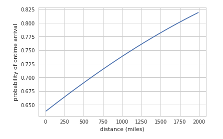
This section displays a plot of how the probability varies as a function of one of the variables by varying just that variable while keeping the other two fixed.
This shows how ontime arrival probability rises with overall flight distance:

There is a small, but positive, relationship there: longer flights are more likely to arrive on time.
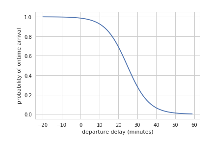
Now compare this to the change in ontime arrival probability as departure time increases while keeping flight distance and taxi-out time fixed.
The probability rapidly falls as the departure delay increases beyond 10 minutes.

The final section of the Jupyter notebook, Evaluate Model, evaluates the model by comparing the predictions to the known arrival times for a section of data that was not used as part of the training data set.
In this section, edit the first cell to define the inputs variable as all_flights-0004-* to match the data shard selection you made previously:
inputs = 'gs://{}/flights/tzcorr/all_flights-00004-*'.format(BUCKET)
Run > Run from this cell.
The first step creates a new DataFrame with a join that now selects the days that are not training days. The total number of flights should match the following table:
+-------+-----------+-----------+------------+------------+
|summary|  DEP_DELAY|   TAXI_OUT|   ARR_DELAY|    DISTANCE|
+-------+-----------+-----------+------------+------------+
|  count|      48961|      48961|       48961|       48961|
A new eval function is created that evaluates the total number of predicted cancellations, using a threshold of 70%, and non-cancellations based on the model as well as the actual correct number of cancellations and non cancellations based on the actual test data sets known arrival times..
This function is then used to assess the model when applied to the entire range of test data. Finally, the total results for the data set are displayed and also the results around the decision threshold of 70%.

The percentage of correct cancellation decisions shows when the model is telling you that the flight will be more than 15 minutes late and the data agrees. This overall correctness percentage is not precisely 70% because that applies to the marginal decision cases and the overall data is swamped by the obvious and easy decisions to cancel (or not) of which there are many more. When you limit the report to the data around the decision threshold point, the percentage of correct predictions of arrival on time (and therefore non-cancellation of the meeting) is closer to 70%.
You can build on these basics to develop and test a range of experimental models for your dataset using this environment. Accurate evaluation of proposed models requires that you develop and evaluate the various models using the complete dataset rather than the single shard used in this lab. Cloud Dataproc allows you to leverage the parallel resources across an entire cluster for this. This is beyond the scope of this lab, but the procedure is explained in detail in Chapter 7, Machine Learning: Logistic Regression on Spark, in the Data Science on Google Cloud Platform book from O’Reilly Media, Inc.